Paul Volcker on the Financial Crisis

Cognitive Dissonance

Cognitive dissonance is a psychological state that describes the uncomfortable feeling when a person begins to understand that something the person believes to be true is, in fact, not true.

Is this a trigger effect for the change in expectations? It appears to be what's happening at the moment in the Irish market (evidenced by Prime Time last night).

Four mega-dangers international financial markets face

Article by Dennis J Snower

Four dangers

The first danger we have witnessed since August 2007: The subprime mortgage crisis gave rise to a liquidity crisis in the international banking system, due to uncertainty about who holds the losses. This is leading to reduced lending to firms and households. But that is not the end of the story, because the reduced lending will lead to reduced consumption and investment. With a lag, reduced sales of goods and services will reduce stock market valuations. And, with another lag, the lower stock market prices will – in the absence of any favourable fortuitous events – intensify the banks’ liquidity crisis.

The second danger lies in the dynamics of U.S. house prices. As more and more U.S. households find themselves unable to repay their mortgages, foreclosures are on the rise, more houses are put on the market, the price of houses falls further – with further lags – this leads to more foreclosures and declines in housing wealth. This dynamic process plays itself out only gradually, as households face progressively more stringent credit conditions and house sales gradually lead to lower house prices.

The third danger results from the interaction between wealth, spending and employment. As U.S. households’ wealth – in the housing market and the stock market – falls, their consumption is beginning to fall and will continue to do so, again with a lag. This decline in consumption is leading to a decline in profits, of which more is on the way, which in turn will lead to a decline in investment. The combined decline in consumption and investment spending will eventually lead to a decline in employment, as firms begin to recognise that their labour is insufficiently utilised. The decline in employment, in turn, means a drop in labour income, which, with a lag, leads to a further drop in consumption.

And that leaves the fourth (and possibly the nastiest) of the dangers, one that concerns the latitude for monetary policy intervention. As the Fed reduces interest rates to combat the crisis, the dollar is falling. This is leading to higher import prices and oil prices in the United States, putting upward pressure on inflation. The greater this inflationary pressure – which is currently in excess of 4 percent – the more difficult it will be for the Fed to reduce interest rates in the future, without running a serious risk of inflaming inflationary expectations and starting a wage-price spiral. U.S. firms and households will gradually recognise this dilemma and the bleak prospect of little future interest rate relief will further dampen consumption and investment spending.

The Live Register

The graphs below show the number of people on the live register. We are currently at a level similar to 1999.Expectations are for another significant change this month. The majority of these jobs would appear to be from the construction industry and you can see the changes in the graphs as construction levels rose in the late 90's to present day, unemployment decreased.

Note: no adjustments have been made for population increases or an increase in foreign labour.

The latest update on the Live Register is due on Friday.

The graph below is from 2006 to 2008. To try your own go here.



This graph below is from 1998 to 2008.



The 90's.



The 80's.

Nobel Thoughts - Joseph Stiglitz

An excellent discussion on CNBC with Joseph Stiglitz.

The clip is 11 minutes long but gives an excellent description of the US through a discussion on savings, investment and consumption.

HERE COMES THE ALT-A CRISIS

This short piece provides an interesting & scary comparison between the sub-prime & Alt-A levels of lending and default. The information has been obtained from the New York Fed and is pretty easy to follow.

The basics are that there is more lending in the Alt-A market for higher amounts a lot of which is for non owner-occupied housing. The lending ratio is up around the 90% mark and defaults are already at 14% which is similar to that of the sub-prime area last year.The credit rating difference between these two isn't that great. The majority of these loan applicants were based on stated income or "liar loans". And, finally, the majority of mortgage resets on the Alt-A's are set to kick in over the next two years.

There are strong comparisons that can be made between America & Ireland.
We also had 100% lending (and more).
Lax lending standards.
The "rent a room" to supplement/increase the mortgage.
Interest only loans; when people finally see the real level of repayments they have to make what will happen?
Negative equity is beginning to kick in for those who have purchased in recent times on a high loan to value rate.

In America, it's easier to file for bankruptcy, hand back the keys and walk away. It's not so easy in Ireland, but that's not to say it won't happen.
What about construction workers who can't afford their mortgages due to lack of work. What's to stop them from picking up tools, moving to Oz where there's a demand for their labour and leaving their Irish mortgage troubles behind them?

Super-Senior Debt : Greed & Avarice

An interesting article on super-senior debt.

First, a brief note of explanation. The concept of super-senior debt was essentially invented by creative bankers about four years ago to refer to the chunk of debt that sits at the very top of the capital structure of a collateralised debt obligation. It is the bit that gets paid off first, before other investors, if the CDO ever defaults. In theory, it makes this debt super-safe; indeed, so secure that rating agencies have been happy to give super-senior CDO debt a AAA tag, irrespective of what lay inside the CDO.

HELOC and 80/20 Mortgages in the US

The next stage in the US mortgage crisis is starting to raise its head.

First of all, we have the 80/20 mortgages. In short, this is a form of 100% financing of which 80% is with the prime lender and 20% is with the second lender at a higher interest rate. These are not subprime, they can be for the Alt-A(good credit rating)and better mortgages allowing people to lend with 0% finance. The problem arises when houses are sold at a loss or foreclosed as the prime lender has first claim on the amounts owed. Write downs for this sector have yet to take place.

Then comes the Home Equity Line of Credit (HELOC). This is where people have released equity in their houses to fund their lifestyle. It has been a big factor in the excess spending in the US. Again, when houses are sold at a loss or foreclosed, there's a big problem for these lenders. Being the third in line to 80/20, there is the potential that these lenders could see a return of zero.

Americans owe a staggering $1.1 trillion on home equity loans and in December 2007, 5.7% of home equity lines of credit were delinquent or in default. What if this number was to rise to 10% in a recession? That's another $110,000,000,000 to write down.

Some more reading.

With the 80/20 (and low interest rates), we saw the basic idea of saving & investing to purchase a house go out the window. People were encouraged to spend rather than save as they could always release equity, with the HELOC, in their rapidly appreciating home to spend more or meet debt payments when needed. This involved fictitious capital being injected into the economy at huge rates. As the various Central Banks tried to correct excessive spending by raising rates, delinquencies and foreclosures rose thus causing the banks to tighten lending procedures and incur write downs. There are further write downs to come and we won't see the end of this until the reset button is pushed and everything is marked to market.

Job Market 2009

Credit Squeeze Explained

This is a great explanation & graphic of the credit squeeze from the FT a couple of months back.

Please Don't Listen To Cramer!

Black Paddy's Day (2) The headlines are not great:

Stagflation

Stagflation is the term used to describe the effects of high inflation, slow economic growth and increasing unemployment. A period of stagflation would have an immediate adverse impact on consumption, production and government revenue.

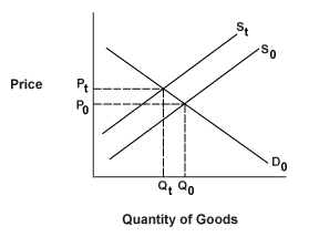
Supply shocks due to natural disasters, adverse weather, war or increases in soft & hard commodity prices can slow economic growth and/or increase inflation. The below diagram illustrates how prices may increase as supply decreases.


This has a direct affect on a households consumption & investment decisions. If inflation is high, the household may choose to consume only essential items such as utilities and food. The production sector could suffer a double blow from low consumption and an increase in raw material prices. This flow will then continue to the governments income from taxes which will be reduced. There is the potential for the stagflation to spiral deeper as the government may raise taxes, the production sector increases prices to maintain profit margin and the household consumes less & less. Additionally, if production levels are low, there is likely to be a cut back on the levels of employment which furthers the likelihood of stagflation.

The monetary policy by the central banks can also be a catalyst for stagflation. A prime example of this is the FED's decision to cut interest rates during the current credit crisis. These rate cuts have a direct affect on the exchange rate of the US dollar. The value of the US dollar has decreased against other fiat currencies, such as the euro (diagram). This makes imports more expensive which again affects household consumption and the resulting flow.



Additionally, the availability of cheap credit by way of low interest rates facilitates inflation as households are more likely to increase consumption than to increase savings due to low rates. Cheap credit leads to an increase in lending which can result in households spending beyond their means or bidding up the price in consumables, hence the inflation risk.

Black Paddy's Day?

Investment banking CDS stress. Watch out this week for the Q1 numbers from the three of Wall Street’s finest left standing. Source





How Debt Bites Back

An explanation of the TAF

Krugman: What’s Ben doing? (Very wonkish) has the FED become a pawnbroker?

Every Change Of Rate

In Europe, Central Banking Is Different

New York Times Article

Blog Work 4. Question 2

Q 2.1
The liquidity preference theory concentrates on the supply and demand for money to explain how interest rates are determined. Keynes considered the desire for individuals to hold their wealth in liquid form as the demand for money. The desire on the part of the individual was called liquidity preference, which was specifically defined as an arrangement of a person’s resources, valued on money or wage units which the person will keep in monetary form in various sets of circumstances.

According to Keynes, liquidity preference determines the actual rate of interest in given circumstances. It fixes the quantity of money, which agents will hold when the rate of interest is given.

M = L(r)

M = quantity of money
L = function of liquidity preference
r = interest rate



If the interest rate is reduced, people will increase their demand for monetary assets.

Keynes identifies three motives for people to hold their wealth in monetary form.

• Transactions motive – the need for cash for current spending
• Precautionary motive – the desire for security for unknown contingencies.
• Speculative motive – to take advantage of a profit making opportunity.

Q. 2.2
Model PC is a good illustration of Keynes’ original vision of decision-making and includes Keynes’ three divisions of liquidity preference, however it may not ultimately be a faithful representation.

Model PC states that the quantity of money held depends on the interest rate of other assets, which represents Keynes’ precautionary demand for money. The rate of interest will influence people’s desires to hold money as security for future contingencies. Model PC also relies on two decisions by households; how much to save and how to allocate these savings. According to Keynes, the marginal propensity to consume will determine how much will be saved and then households must decide in what form their money will be held; in the form of immediate liquidity or savings for a specified or indefinite period.

In the PC Model, the rate of interest equalizes the supply of and demand for bills at the end of the current period, which is the rate of interest for portfolio decisions. Similarly, Keynes maintains that the interest rate is the equalising function in the desire to hold wealth in cash form and the availability of cash.

However, in Model PC agents have perfect knowledge regarding the incomes they will receive, in fact this is how the model is built, the interest rate is also fixed such that r = ˉr with the purchase of government bills. Conversely, uncertainty is a key influence in Keynes’ model. A critical explanation for holding wealth as money is the uncertainty surrounding the future cash value of a holding of bonds and the complex rates of interest for varying maturities that will prevail at future dates. The risk in Keynes’ theory is the risk of capital losses on bond portfolios caused by an increase in interest rates, however Model PC is not concerned about possible capital gains or losses that could arise from changes in the prices of financial assets. Hence, Model PC can be seen to be a slight deviation from Keynes’ original interest rate theory.

Websites:

Reference 1.pdf
Reference 2.
Reference 3.

Government Money with Model Portfolio Choice (PC)

Model PC involves a combination of the circular flow of income approach with the stock approach. This allows us to view money as both "a device allowing transactions between agents to take place" & "a financial asset which agents hold for investment purposes".
A central bank that can offer bills (B) at the rate of interest, r, is also added to Model PC. Using r on an asset, the agent can decide whether it is preferable to hold money or another financial asset.

Note: r is held constant over the entire period of the bond to avoid the inclusion of capital gains on the asset, thus simplifying the model.

Balance Sheet for Model PC

The household has private wealth, V, which is the sum of money, H, and bonds, Bh.
Private wealth is equal to public debt which is held by the Government, +V. This, in turn, is equal to the sum of bonds held by the household and the central bank. This allows all rows & columns to sum to zero.

Transaction Flow For The Economy

To take all transactions into account, the rows & columns each sum to zero.
With this new flow, we must incorporate the bonds issued by the Central Bank (CB) & the payments generated for households as a result of interest payments.

The inclusion of the CB sees a marked change from Model SIM with its capital & accounts components. "Current account describes inflows & outflows that form the current operation on existing assets or liabilities & salaries of CB. Capital account describes changes in the balance sheet of the CB for instance, when it purchases new bills." Additionally, any profits the CB makes are redistributed to the government giving the CB a net worth of zero.

The Equations Of Model PC

(1) National Income: Remains unchanged
(2) Disposable Income: Interest payments on government debts are added to this equation.
(3) Taxable Income: Similar to (2)
(4) Reflects the change in total wealth as a result of the difference between disposable income & consumption.
(5) Consumption function now has total wealth instead of money (SIM) as second argument. It's important the conditions are met or the economy would run out of money.

The Portfolio Decision
The PC model requires that the households decision making process is divided into two stages:
1 - A decision on the proportion to allocate to consumption & saving.
2 - A decision on the allocation of the households acquired wealth during current & previous periods.

The household wants to hold a proportion of their wealth in bonds and the remaining proportion in money. the allocation is decided by the attractiveness of the interest rate. The higher the return on bonds, the higher the proportion of wealth will be allocated.
(6) Describes the amount of money to be held taking into account the interest rate & level of disposable income to wealth.
(7) Describes the amount of bonds to be held using the same weightings as (6) but in reverse.
(8) Balancing condition: 1 = (Hh/V) - (Bh/V)


(9) Government deficit is financed by bills newly issued by the Treasury department.
(10) changes in supply of money equal changes in supply of bonds
(11)Explains how the demand to hold bonds as assets over money is determined with the use of the interest rate(12).

Quotes referenced from Godley & Lavoie, chapter 3, pages 99-107

Homework

Q1 (1)

SIM
• Households know the multiplier process and the parameters of the economy – perfect knowledge.
• Wealth is the equilibrium mechanism.
• Quick convergence rate
• Consumption function: Cd = α1*YD + α2*H-1
SIMEX
• Slow convergence rate – delayed expectations, it takes longer to approach to a steady state solution.
• Introduces imperfect knowledge/uncertainty into the model.
• Households must estimate the income they will receive and the amount of money they wish to hold.
• Households are assumed to have mistaken expectations – if realized income > expected income they will hold the difference in the form of larger cash balances.
• Role of money is the equilibrium mechanism. Money acts as a buffer and provides flexibility when expectations turn out to be incorrect.
• Consumption function: Cd = α1*YDe + α2*H-1

Despite expectations both models achieve the same stationary state.

(2)

Steady state: Y*=G/ Θ
If households’ realized income is higher than expected (W.Nse – W.Nd), households will hold the difference in larger than expected cash balances ΔHs – ΔHd. They will give up more money in the form of taxes (Td – Tse).

Expectations about income will remain unchanged before and after a shock. If actual income is higher than expected, the increase in wealth will be higher than anticipated which will make consumption grow.

In the model, if expected income is lower than realized income, the stock of wealth will grow until the consumption lost through mistaken expectations about income equals the additional consumption out of wealth. Conversely, if expected income is less than realized income, the stock of wealth will fall.

In the real world, people have mistaken expectations and there is a high level of uncertainty particularity in times of recession where people may consume less and save more. When the economy begins to recover, people may then start to consume more than they save. This demonstrates the flexibility people have with their income.


(3)

In period one there is no economic activity and none has existed. The government has injected no money into the economy and households have no income.

In period two the government spends $30, which initiates the economy and circulates within the system.
• Producers pay households 30units of cash
• Households pay 20% in taxes (6 units => YDe=24)
• Households consumption: C = α1.YDe + α2.H-1 (0.6)(24)+(0.4)(0) = 14.4

In period three the government has not injected any extra money into the economy, therefore government expenditure remains at $30.
• Households consumption: C = α1.YDe + α2.H-1 (0.6)(35.52)+(0.4)(21.12) = 30
• Expected income = realized income YDe = YD-1

In the infinite period
• GDP (Y) = G/ Θ = 30/0.2 = 150 Fiscal stance: the stationary level of income
• Taxes 150*0.2 = 30

Question 2.

It is possible to specify a version of SIM that replicates the ISLM model


The IS Curve – Saving & Investment (Goods Market)
Examining the IS curve with the SIM model in mind, we make the assumption that supply must always equal demand. Therefore, the below income equation will fit for supply and demand.

Y = C(Y-T) + I(Y, i) + G

An increase in the supply, Y, would indicate that there is and excess supply of goods. To return this equation to equilibrium, an opposite reaction would have to take place such as a fall in interest rates, i.
The fall in interest rates would be used to encourage a rise in consumption as high interest rates encourage investors to save money due to the high expense of loans or the advantages of investing in bonds.
This relationship is best displayed in the IS curve graph diagram. It can be seen in the graph that as the interest rate (i2) is increased, the output (Y2) decreases i.e. output is a decreasing function of the interest rate.

Given the above equation, and a set interest rate, we can establish that changes in consumption and taxes will shift the IS curve to the left or the right to remain in equilibrium. This is evidenced in the diagram for an increase in taxes.



Increase in Taxes: IS shift left
Decrease in Taxes: IS shift right
Increase in Consumption: IS shift right
Decrease in Consumption: IS shift left

Y: Income
C(Y-T): Consumer spending as a function of disposable income
I(Y, i): Investment as a function of real interest rate
G: Government spending


The LM Curve – Financial Markets
The below equation fits for money supply equals money demand in the SIM model.

M/P = YL (i)

An increase in Y would lead to an increase in the demand for money by households. To maintain equilibrium, it would be necessary for an increase in interest rates to bring the level of demand back to that of supply. This is best illustrated in the diagram of the LM curve where the interest rates are raised to i2 to maintain equilibrium.

Additionally, if there was an increase in the money supply, a cut of interest rates would be required. This would cause the LM curve to shift down.

Increase in Money Supply: Cut in interest rates & shift down of LM curve
Decrease in Money Supply: Increase in interest rates & shift up of LM curve.

Y: Real income
P: Price level
I: Interest rate

The IS-LM Model and some function in SIM

For the IS-LM model, we take the two graphs and combine them. The point at where they meet is the point at which both models achieve equilibrium. The basic theory behind this model is that, as a factor of either model changes, say the IS model for example, the IS model will move up or down along the axis of the LM model to maintain equilibrium.

Td = θ. W.Ns θ<1

From the previous diagram, we can see what happens as taxes are increased. Disposable income is affected which leads to and affect on output, thus the IS curve shifts to the left. As there is no tax function in the LM model, the model is not affected.

However, the change in taxes will have caused a change (decrease) in the interest
rates, as a result of the decrease in income (Y), so the IS model will move along the LM curve to equilibrium. Similar results would show for changes in money supply and consumption.

Stability

We can see from this example that a change in one factor has a direct affect on the IS model to which it is a function of and an indirect impact on the LM model. This shows how difficult it is to use just one policy to have the desired affect on the overall economy (and of course SIM).

Td :Tax demand
W.Nd :Wage rate times employment demand
Θ: proportion of change

References
Macroeconomics, Blanchard. Chapter 5
Monetary Economics, Godley & Lavoie. Chapter 3
Wikipedia
Egiwald
Roubini & Backus
MIT (.pdf)